Check also:
Measurement scales
There are four basic levels of measurement:
- Nominal scale
This is the lowest level of measurement in which a unit of analysis is assigned to a specific category of variable. The categorisation must fulfil two conditions: to be exhaustive and to be mutually exclusive. Consequently, each observation must be assigned to a single category appropriate to it. Examples are gender, colour or country of birth. However, there is no order or hierarchy within the assignments to the groups. Symbolically, we often assign them consecutive numbers, e.g., gender (1 - female, 2 - male), but this does not entitle us to perform algebraic operations on them.
A special case of nominal level of measurement is the dichotomous variable, i.e., zero-one coded variables, e.g., exam success (pass/fail). Multiple-choice questions can also be dichotomously coded, where each possible answer will be a separate variable. Although, from a theoretical point of view, we can say that, for example, the category pass is better than fail, in practice we cannot consider dichotomous variables in the context of a hierarchy.
- Ordinal scale
This level of measurement allows data to be ordered according to a specific hierarchy. It assumes that the intensity of a variable is a continuum on which the different categories of the variable can be ordered. One such example could be the degree of difficulty of the task at hand (easy, medium, difficult), or the level of education (from early childhood to higher education). In this case, however, it is necessary to make sure about the nature of the data; if it turns out that the categories include particular types of schools (general secondary, technical, vocational), then this variable will be measured on a nominal scale, as it is not possible to logically assign an order to the categories.
The ordinal scale allows for an indication of the intensity of the phenomenon under study, i.e., that a particular observation is larger, older, requires more resources, etc. From the point of view of the analyses themselves, it does not matter whether the order is ascending or descending. What matters is that there is a logical succession of categories.
The Likert scale is another example of an ordinal level of measurement. Often used in psychology and sociology, it is characterised by the respondent's attitude to a given statement through the use of a scale, usually 1-5 or 1-7. For example:
Statement: Company X's products are innovative.
Answer:
- Strongly agree
- Agree
- Have no opinion
- Disagree
- Strongly disagree
By analysing the results later as a group, we can therefore get an answer to the question of which company's products are considered more innovative. However, it is not possible to determine from this how big the difference in this innovation is.
- Interval scale
With the interval scale, we can compare data with each other and determine the difference between them, in other words, measure their distance from each other on the scale used. The numerical values of the individual variables are therefore no longer merely symbolic. However, the interval level of measurement will still not have an absolute zero. A good example of this is the measurement of temperature on the Celsius scale; if yesterday was 10 °C and today is 10 °C more, we will know without much effort that today is 20 °C. However, can we say that it is twice as warm? We could probably make a guess that it is, but what if the starting temperature was -5 °C?
The interval scale therefore allows us to find out by how much the individual values differ.
- Ratio scale
This is the most accurate level of measurement. This is because the ratio scale allows you to determine (as the name suggests) by how many times the different values differ from each other. Going back to the previous example, in order to measure temperature on a relative scale, the Kelvin scale must be used. It is called an absolute scale because it contains an absolute zero. Although it is only a theoretical assumption (according to physics, it is the state of cessation of all vibrations of molecules which is impossible to achieve in practice), temperatures expressed on this scale can already be freely compared with each other, e.g., 20 K will be twice as much as 10 K.
Another example is the age of a car. If it is presented as the vintage of the vehicle (e.g., 2019, 2023, etc) then this variable will be measured on an interval scale; we can determine the difference in the age of the cars because the zero on this scale is only conventional (it starts 'our era'). However, if we choose to present this information in years, then we can assume that a car driven straight off the production line is 0 years old, while one manufactured in 2019 will be 4 years old as of today.
Qualitative and quantitative variables
It is worth briefly mentioning at this point the division of variables into qualitative and quantitative variables. Qualitative variables include variables measured on nominal and ordinal scales. They have specific categories, the breakdown of which is exhaustive and mutually exclusive (as mentioned earlier).
Quantitative variables, on the other hand, have properties that we can measure precisely. The scales that make this possible are the interval and ratio levels of measurement. Working in PS IMAGO PRO, these two types of measurement scales are treated as a single measurement level group.
The analyst therefore has a choice of three scales: nominal, ordinal and quantitative. It is important that the level of measurement is appropriately assigned to each variable, as this will be crucial in subsequent analyses. Every statistical test has its limitations and it is not uncommon for these limitations to relate precisely to the way in which variables are measured.
Discrete and continuous variables
Another division, in terms of the level of measurement that can be encountered, is the distinction between discrete and continuous variables. Discrete variables are those variables that take a finite number of values. These values can be assigned integer natural numbers and, at the same time, no other values can be found between two 'adjacent' discrete values. In practice, such variables are usually those measured on a nominal or ordinal scale, e.g., with eye colour (1 - brown, 2 - blue, 3 – other), we cannot logically assign an observation a value of, say, 2.5.
However, there are also quantitative variables that can be classified as discrete. Examples include the number of children in a family, passengers on a ship, or scores on a test with yes/no questions. Due to the nature of such variables, the set of their values is finite and it is not possible to logically justify a non-integer number here.
Continuous variables, on the other hand, can take on arbitrary values, sometimes within a limited (mainly by the laws of nature) range, e.g., if we are studying the height of people or the temperature of the environment. Between two values, however, we can observe infinitely many other values. Here, the only limitation is the accuracy of the measurement at our disposal.
Levels of measurement and statistics
As mentioned earlier, the level of measurement can be a certain constraint when choosing the statistics to be calculated. Let us now look at one of the most basic descriptive statistic, central tendency.
As you might guess, the nominal scale has the most limitations. We can calculate the mode for it, but the mean or median is not available, e.g., returning to the example with eye colour, we can say which value was most frequently observed (dominant/modal), but because the categories are not ordered, neither the middle of the range (median) nor the 'average' value (mean) of eye colour can be calculated.
If the variable is measured on an ordinal scale, in addition to the mode, the median can also be calculated, e.g., when analysing a variable relating to the respondents' current stage of education, the dominant category may well be the primary school stage (the longest period of schooling and therefore the most children), but the median will be the secondary school stage category. We can therefore obtain both information about the dominant category (in terms of numbers) and which category is in the middle of the range in our sample group. The mean remains an unavailable to us.
Quantitative scales make it possible to calculate all three statistics. The above information is summarised in Table 1.
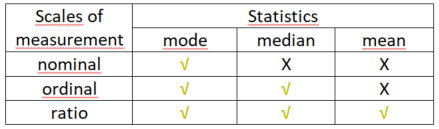
Table 1. Availability of selected statistics
for each level of measurement.
The limited ability to calculate statistics also translates into the availability of statistical tests. Knowing the theoretical basis of the various methods of data analysis, we will know whether they can be applied to the dataset we have. If we know, for example, that analysis of variance is based on mean values across groups, we will also know that the dependent variables we want to use for such a test must be measured on a quantitative scale.
There are, of course, also statistical tests designed to analyse qualitative variables. An example of this is the chi-square test[1], for which the basic underlying statistic is the count in the individual groups.
Summary
Level of measurement is an important property of any variable, and its proper assignment to each variable at the data creation stage is crucial if further analyses are to be reliable and relevant.
Although familiarity with statistical tests and their theoretical underpinnings greatly facilitates the analyst's work, hints provided by statistical software can also be useful: when selecting variables for analysis in PS IMAGO PRO, it will provide information that a given level of measurement cannot be used in the given procedure. When working with data, we can also perform transformations that divide our data into certain groups, e.g., for the purposes of a desired statistical analysis, we may transform age expressed in years (quantitative scale) into a specific number of age groups (ordinal scale, e.g. 18-30, 31-50 and 51+). In special cases, we can create a new ordinal variable on the basis of a nominal variable. An example of this would be to convert the names of the schools attended by the respondents into categories of educational stages, for example, IV Catering Technical School into the secondary education group, all primary schools into primary education category, etc. Usually, however, it is simpler to 'step down' from the more precise levels of measurement to the more basic ones. While this gives the analyst some flexibility, understanding the problem of measuring a variable will protect the researcher from slip-ups such as calculating the average of a province or field of study, and make it easier to choose analyses in the context of the data at hand.
[1] https://en.predictivesolutions.pl/pearson-s-chi-square-test-of-independence,en