To begin with, it is worth recalling the basic information about Pearson's chi-square test. The first one, which is probably the most commonly used when we talk about this kind of test, is the chi-square independence test. In various types of survey research in the field of marketing, psychology or sociology, the main type of variables that the analyst has at his/her disposal are qualitative variables. A popular test used to analyse two qualitative variables and determine whether there is a statistically significant relationship between them is the chi-square independence test.
We can use the chi-square test of contingency when we have a single qualitative variable. Often, but not always, the analyst expects the categories to have equal proportions, e.g., when we use a t-test for independent groups or in the case of analysis of variance. The test allows us to check whether the frequency distribution of a categorical variable differs significantly from our expectation. In other words, the chi-square test of contingency is used to assess whether the empirical distribution of the data is consistent with the theoretical distribution that is described by a specific null hypothesis.
A similar form of test is the chi-square test of homogeneity, which checks, for example, whether two distributions of a variable have the same proportions relative to each other. In general, the chi-square test of homogeneity is used to check whether the frequency distribution of a categorical variable differs from another defined distribution. This test is used when the researcher wants to check whether there is a significant difference between the distributions of at least two categorical variables. Examples of null hypotheses that can be tested using the chi-square test of homogeneity include the frequency of a certain event in different groups, a comparison of consumer preferences for different products, etc.
From a mathematical point of view, it is worth noting that these are actually the same tests. However, we often think of them as different tests because they are used for different purposes.
Chi-square test formula
The formulae for the homogeneity test and the contingency test are in the main very similar to each other. In both cases, the calculation of the chi-square statistic is based on observed and expected values.

where:
![]() – chi-square test statistic,
– chi-square test statistic,
![]() – observed values,
– observed values,
![]() – expected values,
– expected values,
![]() – number of measurements/groups.
– number of measurements/groups.
As can be seen, the formula is similar to that for the chi-square independence test. The greater the difference between the observed and expected values, the greater the value of the chi-square statistic will be. To decide whether the difference is statistically significant, compare the resulting test value with the table of critical values of the chi-square distribution.
Example of calculating a chi-square statistic
We asked respondents if they did any physical activity at least once a week, e.g., running, gym, cycling. We received the following results:
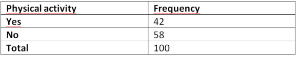
Table 1. Engaging in physical activity at least once a week
We want to answer the question of whether the difference between people doing at least one physical activity per week and non-exercisers is statistically significant. To do this, we will calculate the chi-square statistic. The easiest way to do this is to use a properly prepared table.
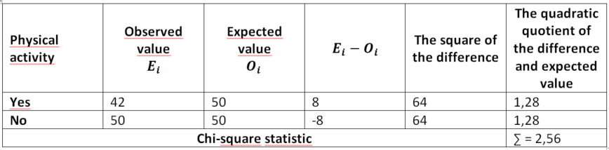
Table 2. Calculation of chi-square statistics for physical activity data
Having calculated the chi-square statistic, we still need to calculate the number of degrees of freedom (df) to answer the question posed above. The formula for the number of degrees of freedom is as follows:
df = k-1
where:
k – number of categories.
In our example, the number of degrees of freedom is 1.
Then compare the chi-square value with the table of critical values of the chi-square distribution. Assuming a significance level of 0.05, in our example the chi-square test showed no statistically significant difference between exercisers and non-exercisers.
Chi-square test of contingency as a measure of variation for qualitative variables in PS IMAGO PRO
In this material, I have discussed the basic issues of the chi-square test of contingency and how we can calculate it without using a computer and statistical software. Let us now turn to a non-obvious application of this test, namely to use it as a measure of variation for qualitative variables.
Let us return to the example of people exercising. If the numbers of exercisers and non-exercisers are the same, the value of the chi-square test will be 0. The same will be true if the variable under analysis has more than two categories for which the counts are the same. If the value of the test is close to 0, then the variation in the categories of the variable under study can be interpreted as small.
The minimum value for the chi-square test is 0 when the distribution of the abundances is uniform. The maximum value, on the other hand, is reached when all observations are assigned to one category of the variable.
One of the procedures that allows the chi-square test statistic to be calculated in PS IMAGO PRO is Data Audit. The procedure allows you to prepare a summary for the analysed variables in the form of tables containing selected statistics broken down into qualitative and quantitative variables.
Let us analyse another example in which we have a variable with four categories.

Table 3: Distribution of the variable "Type of car body".
Analysing Table 3, it is immediately noticeable that the counts for each category are not equal, thus there is variation between the categories. Using the Data Audit procedure, let us check what the value of the chi-square statistic is.
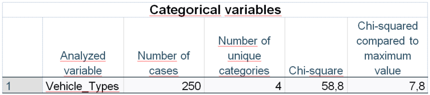
Table 4. Chi-square results for the analysed variable
As can be seen, the test value is significantly greater than 1 and is 58.8. As this is not a value standardised to a specific range, it is difficult to determine whether this is a large value or not. One would have to calculate the maximum value for this statistic each time for a specific example. The data audit makes this task easier, as it allows you to calculate what percentage of the maximum chi-square value for this example is the value that was calculated (the 'Chi-square compared to maximum value' column). In our study, it represents close to 8 per cent - meaning that for this variable and this data distribution, it is 8 per cent of the maximum variability that the variable can take.
In summary, chi-square tests are popular tests applicable not only when looking for relationships between qualitative variables, but also when we need to check whether the categories of a qualitative variable are collinear. Often, many statistical tests require the assumption for a grouping variable that its categories are equal (e.g. one-way ANOVA). The chi-square test of contingency is a useful statistical tool for comparing the frequencies of different categories of a qualitative variable and assessing whether there are significant differences between them. Another use of this test is to use the chi-square test of contingency as a measure of variation for qualitative variables. In addition to the statistics already presented on the blog such as Entropy and Gini Index - also available in PS IMAGO PRO - the Data Audit procedure and the chi-square statistic can be a very good complement to the prepared statistics needed when analysing the distribution of qualitative variables.