Translating this into action, neural networks can be used in areas such as production control systems, sales and price forecasting, identification of high-value customer segments, speech synthesis, handwriting recognition and even criminal profiling or dangerous cargo detection at airports.
The algorithms in question here are, to be precise, artificial neural networks (ANNs). Their operation is inspired by natural neural networks, or simply the nervous system which is made up of billions of neurons that form huge networks of connections with other nerve cells. Through these connections, known as synapses, the neurons transmit signals to each other, thus enabling them to process information and generate appropriate responses. The most active connections are strengthened, or, 'learn' to perform specific tasks and thus form specialised networks within the nervous system.
The functioning of the brain is still an unsurpassed model for the operation of computers, but the development of artificial neural networks is allowing their use on an increasingly large scale. Although they can be even more efficient than the human brain in certain tasks, such as mathematics, tasks such as distinguishing between types of animals or material textures can be very computationally intensive and the results obtained will not always be correct.
Construction of an artificial neural network
The basic unit of artificial neural networks are neurons. They form at least three layers in the network:
- input layer – each variable used in a given neural network will have a corresponding neuron in this layer; the neurons of the input layer only take on the values of a single variable (or a single category in the case of qualitative variables) and, without modifying them, pass them on to the next layer,
- hidden layer – is responsible for receiving values from the previous layer, processing them and passing them on to the next layer; there can be many hidden layers, and the number of their neurons depends on the user – the more neurons, the greater the computational power and flexibility of the network, but the risk of overfitting the network also increases,
- output (result) layer – combines all the values from the last hidden layer and passes on the final value in the form of one neuron for a quantitative variable or as many neurons as the number of categories the qualitative variable has.
But how exactly are networks created within these layers and the neurons that make them up?
Each neuron of a layer is connected to all the neurons of the next layer. In unidirectional networks, which we will focus on in this article, there are no connections between neurons within a layer and there is no possibility of a connection bypassing the next layer (e.g., a direct connection between the neurons of the input and output layers). However, there are neural networks with a more complex structure, e.g., recurrent networks that allow for the possibility of feedback-like connections.
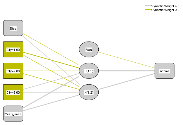
Figure 1. Example of a unidirectional neural network with one hidden layer
Neuron action
The rules of a single neuron depend on its role in the neural network. As we already know, the neurons of the input layer have a simple task - to transmit the value of a given variable to the neurons of the hidden layer. If the variable is quantitative, one neuron corresponding to it will be present in the network and will take the corresponding numerical value, e.g., the number of years of cooperation with a customer. In the case of a qualitative variable, each of its categories will be assigned one neuron, transmitting a zero-one value, for example, if we have customers from three different cities (where 1=Kracow, 2=Warsaw, 3=Wroclaw), and the network will analyse the case of a customer from Krakow, then the neuron in which City=1 will take the value of 1, while neurons where City=2 and City=3 will take the value of 0.
In the next layers, i.e., hidden and output layers, the principles of neurons are slightly more complicated. Most of the neurons in these layers combine input values from the neurons of the preceding layer and apply a so-called activation function to the combined input values. In addition, each connection between neurons is assigned a weight; the higher the weight, the more the value of a given neuron influences the end result, i.e., the final value of the resulting layer (Figure 2). In our example, it may turn out that the greatest weight for the neurons of the hidden layer will not be how many years the cooperation with the client has lasted, but what city he or she is from, or, even more specifically, whether the client is from Warsaw or not.
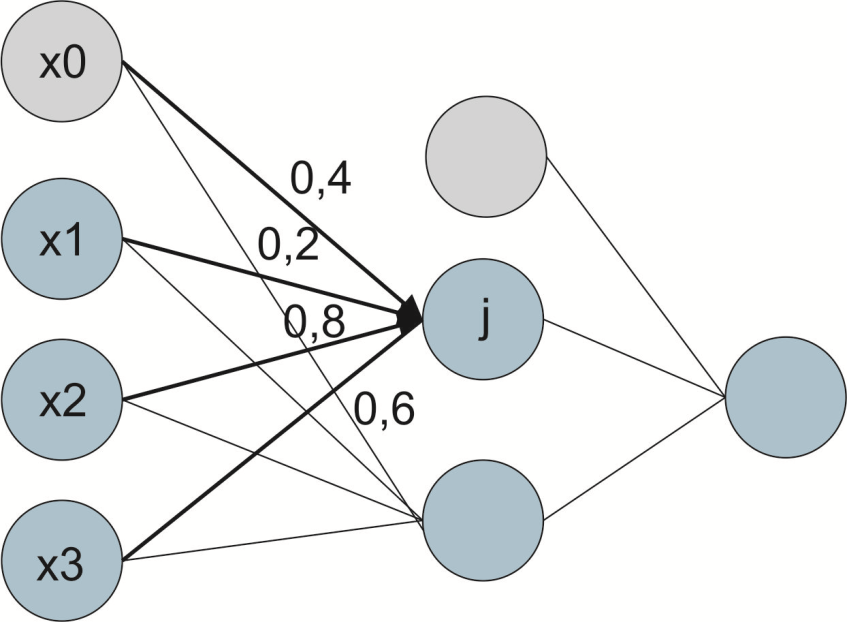
Figure 2. Example network diagram with synaptic weights
The combining of input values within a single neuron is done by means of a so-called combining function. This is usually the sum of the values of the neurons of the previous layer multiplied by their corresponding synaptic weights.
The value that a neuron will take (and pass on, if it is not already a resultant layer) depends on the activation function. We will not go into its intricacies in this article, but it is worth mentioning that the most popular activation functions are, for example, the logistic function and the hyperbolic tangent.
The operation of the activation function is shown in Figure 3. The blue circle is a combining function, calculated from the values of the neurons of the previous layer - x, taking into account their individual weights - w. The result of this function is the value of the neuron - y, which for the neurons of the next layer will be one of the values of x.
However, if it were a diagram of the neuron from the output layer, y will be the result of the whole neural network, which the analyst will receive.
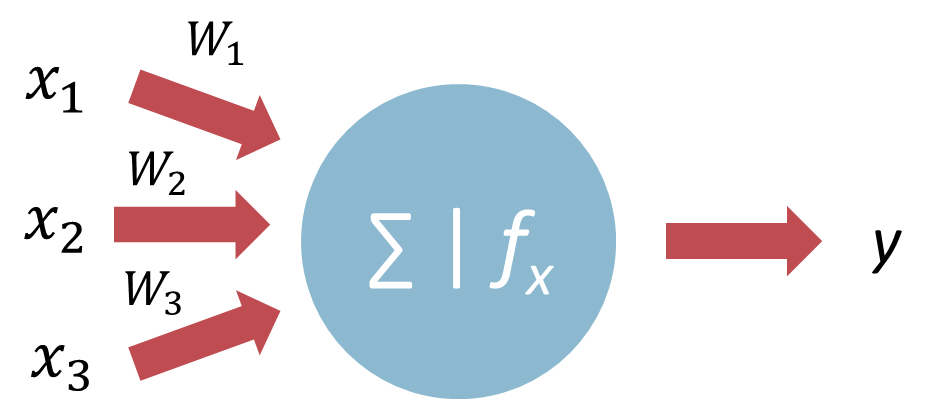
Figure 3. Activation function diagram
In Figures 1 and 2, an additional type of neuron can be seen, the so-called loaded error, which represents the possibility of error. These neurons appear in the input layer and the hidden layers. By including such a load, even if zero-sum information has been received by the neuron, it will pass on a certain value. In this case, it will be equal to the value of the error neuron of the previous layer.
Network learning
So let's go back to our example in Figure 1 and consider how a neural network can predict the revenue from a contract with different customers based on the years of cooperation and their location (Krakow, Warsaw, Wroclaw). It is already intuitive to guess that in addition to having data for the input variables, it is also good to have some data for the target variable (from the output layer). The neural network, on the basis of the information it has on the characteristics of the customer and what revenue is generated by cooperation with them, will be able to predict what revenue can be counted on with a given customer profile. This can help to determine the company's growth strategy, e.g., it may be more lucrative to take care of long-standing customers from the capital, or to predict revenue in future years, depending on which customers we have been able to establish and continue working with.
Network learning is done by adjusting the weights. At the start of the process, weights are chosen at random and then the network, in subsequent learning steps, adjusts the values of the individual synaptic weights to increase the probability of correctly estimating the outcome variable (i.e., reduce the prediction error). This process can be very time-consuming, especially for large collections. In order to make the best use of the resources available, both the amount of data held and the computing power, the following types of learning can be applied:
- whole set – weights are updated on the basis of the entire dataset; best minimises overall error, but requires multiple repetitions, hence best suited for small datasets,
- individual – the weights are updated on a record-by-record basis, i.e., for each observation in turn; this method works best for large datasets,
- subset – the set is divided into equally sized subsets, and the weights are updated after the algorithm has passed through one group; this compromise between the first and second type of learning is recommended for medium-sized sets.
Just as important as optimising the learning of the network is controlling whether overlearning occurs. This is a situation in which a neural network becomes so 'focused' on the dataset being used that it ceases to be universal. Such an overlearned network will learn "by heart" its first dataset and within that, the results will predict perfectly. If, on the other hand, we were to add new records to it (in practice, we know that these may not necessarily be fully consistent with the existing data), the prediction of their value of the target variable could be completely wrong.
To prevent this from happening, a subsetting is done before the learning process starts. The main set is the learning set – based on this, the number of neurons and their connection weights will be determined. At the same time, the number of erroneous results is verified on the basis of the testing set. By design, each adjustment of the weights after their random assignment should result in fewer errors, regardless of the dataset. If, at some point, a decrease in the number of errors is only noticeable in the learning set, it means that the network is starting to overlearn, instead of learning to generalise the relationships. The resulting model can be verified on the last subset – the validation set. Here, the predicted values are compared with the actual values – using records that were not previously involved in the learning process at all. In this way, the accuracy of the model can be verified. The validation dataset can be dispensed with in some cases, as it limits the number of data on which the network can learn.
Summary
Artificial neural networks are information processing systems that will perform well in tasks such as prediction, classification, or clustering. On the basis of a provided dataset, they learn to perform a specific task, and the resulting model can later be generalised, i.e., used on other datasets with variable data. An important advantage of neural networks is that they are not very restrictive in terms of the nature of the data used. Larger amounts of data for learning are obviously preferred by the network, but it can even be used for smaller data sets.
The extent of supervision of the model building and learning process of a neural network is largely up to the user. He or she can define only the independent variables (factors and co-variables) and the dependent variables (targets), but aspects such as subsetting, network architecture (number of layers, number of neurons, type of activation function, etc.), type of learning, or even stopping criteria (e.g., time, or maximum number of steps without error reduction) can be modified if necessary.
Such a high degree of flexibility of artificial neural networks makes their application really broad, which the current dynamic development of artificial intelligence emphatically confirms.