An analyst or statistician can use the variance and several related methods to efficiently answer the question of whether the average values are close to each other, or whether they are characterised by much greater extremes.
Variance
Variance is one of the basic measures of the dispersion of observed results, and is deployed in many, even very sophisticated, analytical techniques. Measures of dispersion, otherwise known as measures of spread, dispersion or variability, allow the variation of the values of a characteristic around central values to be determined: the more the results are clustered around a central value, i.e., the mean, the less the dispersion of results, and the smaller the measures of variability.
The variance is the arithmetic mean of the squares of the differences between the individual values of a variable and its arithmetic mean for the whole sample, i.e., the mean of the squares of the deviations from the mean. It can be written as a formula:
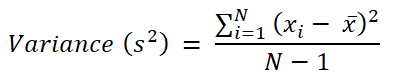
The variance can be interpreted as the average error that will be made when predicting the value of a variable based on its mean. So let's look at how this measure can be used with a concrete example.
We want to compare two departments in our company where the average age of employees in both departments is equal (40 years of age). However, if we look at the individual values (Table 1), we find that in one department the age of the employees varies considerably more.

Table 1. Summary of observations
If we were to rely only on the mean as a measure of central tendency, the information we have about the groups analysed would certainly not be exhaustive for drawing more detailed conclusions or predicting the age of individuals with satisfactory accuracy. The aforementioned measures of dispersion come to the rescue here.
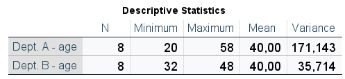
Table 2. Descriptive statistics
Thanks to the variance (Table 2), we obtain the information that in Department A the results were more scattered with respect to the mean than in Department B. By predicting the age of each employee based on the average of the whole department, the average forecasting error will be larger for Department A.
As the variance is calculated by squaring the value, its result cannot be negative. In the case of constant variables, i.e., variables that take the same value for all observations, the variance is 0.
However, the fact that the result obtained is expressed in units of the variable squared is a certain limitation of the variance. Looking at Table 2, we cannot say that the average error in predicting the age of employees in department A is 171 years! So how do we deal with this problem? The standard deviation comes to the rescue here.
Standard deviation
The standard deviation is also a measure of dispersion, and therefore provides information on how dispersed the analysed data is in the distribution relative to the mean. The standard deviation is directly linked to the variance, and its formula is the square root of the variance value:
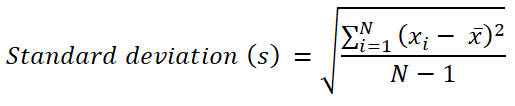
Standard deviation is a more convenient measure in the context of reporting. Its result is expressed in units of the variable being analysed, which makes it possible, among other things, to determine the size of the average error made when predicting using the mean value.
Returning to the earlier example, the standard deviation is obviously larger for Department A (Table 3), in line with the variance values mentioned earlier. In addition, we are further informed that in Department A the results differed on average by about 13 years from the mean, while in Department B the error was about 6 years. At this point, however, it should be noted that the standard deviation is based on the square root of the total number of observations (N) minus one, meaning the interpretation of this measure in the context of the average error made loses some precision.
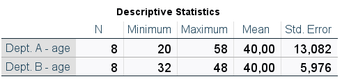
Table 3. Descriptive statistics
Covariance
Covariance is another measure based on variance. Unlike variance, this measure looks at two variables rather than one. Covariance is a measure of the linear relationship between two variables: it examines whether the deviation of values from their mean is similar for the two variables.

Covariance is an unnormalised measure of joint variability, which means that it does not have a defined, fixed range of accepted values. In addition, its value depends on the units of the variables analysed, so it is difficult to determine from this whether a relationship is weak or strong. A covariance value of 0 indicates the absence of a linear relationship between the variables.
In the next stage of our study, we want to analyse the length of service of our company's employees. One of the correlates we can take into account is age. The results of covariance equal to 46.8 (Table 4) confirm that there is a linear relationship between these two variables.
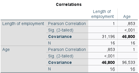
Table 4. Covariance value from the correlation table
Unlike variance and standard deviation, covariance can also take on negative values. This allows the direction of the relationship to be determined: if the value of the covariance is positive, when the value of one variable increases, the value of the other variable increases. If the covariance has a negative value, an increase in the value of one variable will cause a decrease in the value of the other variable. As expected, in the company we analysed, the relationship between employee age and length of service is positive: the older the employee, the longer they tend to work for the company.
Dividing the result of covariance by the product of standard deviations of the analysed variables, we obtain a standardised measure - Pearson's correlation coefficient (r), about which more later. This measure also allows us to analyse the relationship between two variables, but in addition to determining the existence of a relationship and its direction, it also gives us information about the strength of that relationship: we can determine if it is weak, moderate or strong (hence the standardised measure).
Least squares method
Based on the measure of the standard deviation, and therefore the variance, the method of least squares can be used. This method allows us to fit a linear model to the data and, amongst other things, to estimate a linear regression equation.
The method of least squares involves fitting a straight line (or ‘line of best fit’) to a set of data points in such a way that the sum of squares of the differences between the actual and estimated values is as small as possible, or, in other words, to make the straight line run as close as possible to each of the points on the scatter plot (Figure 1).
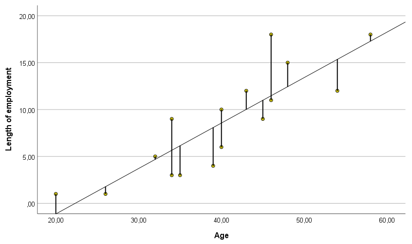
Figure 1. Scatter plot with line of best fit
Some points (actual values) will be above and some below the line of best fit (estimated values). However, the average of the values of these residuals will always be 0. In this way, the predicted values will neither over- nor underestimate the actual observations.
The actual values are also called empirical and the estimated values are called theoretical. The idea of the method of least squares is to minimise the equations between these values, and the straight line determined in this way will be a better fit than any otherwise drawn straight line (for example, from Figure 2).
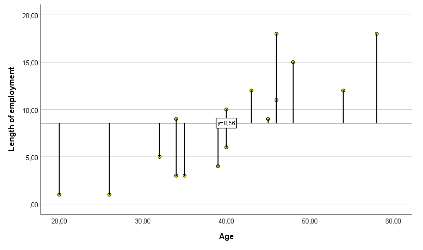
Figure 2. Scatter plot with fit line based on Y mean
We already know that in our company study there is a linear relationship between employee age and length of service. If we wanted to predict length of service based only on an average of 8.56 years, we would be quite wrong, as the predicted values at this data point are highly variable (Figure 2). In other words, we would predict that each person has been working for the company for about 8½ years.
However, if we use the age variable together with the method of least squares, our predictions will be much more precise: a person aged 30 will have worked for us for about 4 years, but for an age of 45 it will already be approximately 11 years of seniority. Of course, in some cases we will be wrong in favour or against individuals, but the error will be much smaller than when using the average.
Summary
The variance is not only a measure of dispersion that allows us to assess the spread of the results, but also a measure with which we can calculate many other, often more advanced measures, coefficients, or use in additional statistical methods. The standard deviation, covariance, Pearson's r and the method of least squares, make it possible, from a simple measure of dispersion, to analyse the linear relationship between variables, or to build a linear regression model that can predict the value of the analysed variable.