General Linear Models
General Linear Models (GLMs) form the basis of several statistical tests, including analysis of variance (ANOVA), analysis of covariance (ANCOVA) and regression analysis. Contributions to the development of GLMs are attributed to many researchers. However, a key role is often attributed to Ronald Fisher. His work on analysis of variance, experimental design and parameter estimation methods was fundamental to GLM. In addition to Fisher, other researchers such as Jerzy Neyman, Egon Pearson and Karl Pearson also influenced the development of the GLM through their work on statistical theory and data analysis methods.
Similar to the linear function, well known from linear regression, general linear models can be succinctly written in the form of the formula:
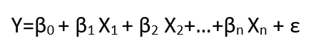
Where:
In short, GLMs include models in which the dependent variable is a linear combination of independent variables. In GLM models, errors are assumed to have a normal distribution and to be independent and homoscedastic. This means that the errors have the same variance for each independent value and are independent of each other.
In general linear models, the analyst pays attention to a number of assumptions that should be met in order to use this kind of statistical tests. However, in reality the data may not always meet these assumptions. For example, errors may be correlated or have a distribution other than normal. In such situations, generalised linear models are used, which allow greater adaptability to different types of data.
Generalised linear models extend the classical GLM by allowing for different error distributions and different combination functions for the relationships between variables. This allows them to be better adapted to a variety of data types and more complex relationships.
Assumptions for general linear models
Let us take a closer look at the assumptions for general linear models in order to know in which situation this kind of statistical toolkit can be used. It is worth bearing in mind that these kinds of assumptions have already appeared when discussing, for example, linear regression or analysis of variance. The basic point to remember is that general linear models are used when the dependent variable is continuous and assumed to have a normal distribution.
The main assumptions of general linear models include:
- Linearity – all these methods assume that there is a linear relationship between the independent variables and the dependent variable (in regression) or between the dependent variable and group effects (in ANOVA and ANCOVA).
- Normality of the distribution of residuals – for linear regression, ANOVA and ANCOVA, it is assumed that the residuals (prediction errors) have a normal distribution. This assumption is important for the validity of the statistical tests and the reliability of the conclusions.
- Homoscedasticity – all methods assume that the variance of the residuals is constant across levels of independent variables or between groups. In regression, it is important that the variance of the residuals is constant with respect to the values predicted by the model.
- Noncollinearity – in multivariate linear regression, it is important that the independent variables are not highly correlated with each other. This could lead to problems in the estimation and interpretation of model parameters.
- No autocorrelation of residuals – the residuals of the model should not be correlated over time.
These assumptions are fundamental to most classical statistical tests and are key to assessing whether a method is suitable for analysing the data collected. If any of these assumptions are violated, this can lead to errors in estimation, hypothesis testing and statistical inference in general.
Generalized linear models
Generalized Linear Models (GLZ) are an extension of classical general linear models. They are designed to analyse data that do not meet standard assumptions, such as the normality of the distribution of the dependent variable. These models were formulated by John Nelder and Robert Wedderburn in 1972. They allow the use of different types of probability distributions (e.g., binomial, Poisson, gamma), which makes them suitable for many practical applications.
Let us turn to the details. The generalised linear model extends the general linear model such that the dependent variable is linearly related to the factors and co-variables via a specified linking function. The model further allows the dependent variable to have no normal distribution. Due to their very general form of the model function, they include many statistical tests and models, such as logistic regression for binary data, log-linear models for count data and many other statistical models. Generalised linear models are not suitable for modelling binary data (e.g., success, failure) or count data (e.g., number of occurrences of an event). In such cases, generalised linear models, such as a logistic regression model for binary data or a Poisson model for count data, will be more appropriate.
The main features of generalised linear models include:
- Linking function: the GLZ introduces the concept of a linking function that transforms the predicted mean values of the dependent variable so that they are linearly related to the independent variables.
- Distribution of the dependent variable: the model allows that the dependent variable may have different distributions from the group of exponential distributions.
- Estimation method: the model parameters are usually estimated using the maximum likelihood method, which differs from the traditionally used least squares estimation method in general linear models.
Comparison of generalised linear models and general linear models
Generalised linear models are primarily more flexible. They can be used in cases where the distribution of the dependent variable is not normal, which may be typical for counts, occurrences, survival times or binary data. General linear models are limited to situations where the dependent variable has a normal distribution, which is more typical for continuous and symmetric data.
Another point about statistical assumptions is that GLZs do not require the rest of the model to have a normal distribution. This makes them more useful for analysing data that do not meet the classical assumptions. General linear models, on the other hand, rely on the assumption of normality and homoscedasticity of the residuals, which can be a limitation when analysing more complex data.
A final difference between GLZ and GLM is the estimation method. Generalised linear models use the maximum likelihood method, which works better with non-normal data. Generalised linear models, on the other hand, use the least squares method, which is efficient and simple to implement, but requires assumptions about the distribution.
The table below compares the key differences between general linear models and generalised linear models.
|
Feature |
General linear models (GLM) |
Generalised linear models (GLZ) |
|
Data distribution |
Data that are normally distributed |
Data that can have different distributions (binomial, Poisson, gamma, etc.) |
|
Estimation methods |
Least squares method |
Maximum likelihood method |
|
Statistical assumptions |
1. Normality of the distribution of the residuals |
1. Distributions from the exponential family |
|
Typical applications |
Analysis of data where the dependent variable is continuous and symmetric. |
Analysis of data where the dependent variable may not be continuous or symmetric, e.g., numeric data, time to event, binary data. |
Table 1. Comparison of key differences between models
GLZs are used not only when the data do not have a normal distribution, but also for other deviations from the assumptions of the classical GLM and for specific data types such as binary or count data.
Example of the use of generalised linear models in PS IMAGO PRO
In PS IMAGO PRO, the data analyst has access to a wide range of statistical tests and models. According to needs, the user can select a specific statistical test or use a separate procedure designed for generalised linear models. In this procedure, the user has access to a wide range of settings and parameters to prepare a model suitable for the data.
Generalised linear models can be used in the analysis of data for a wide range of applications whether in business, medicine, biology or the social sciences. Let us look at a simplified example of the application of GLZ in the context of forecasting product sales depending on various factors.
Suppose we are commissioned by a product manager in a retail company to carry out an analysis to better understand how different factors affect product sales. In this case, a generalised linear model can be used, where product sales are the dependent variable and various factors such as price, promotions, and seasons, are predictors.
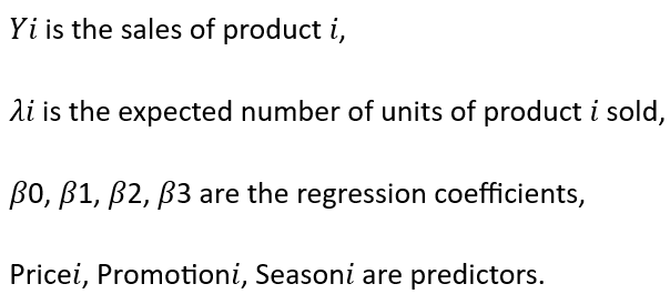
This model may look as follows:
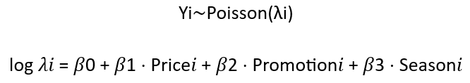
Where:
Why choose generalised linear models in this example? Using a generalised linear model, we can analyse how changes in product price, promotions and season affect sales by assuming a Poisson distribution and a logarithmic linking function in the model. The Poisson distribution is often used to model discrete variables, such as the number of events. This may be appropriate in the context of forecasting product sales, where we are interested in predicting the number of units sold at a given time.
If the assumption is that the number of product units sold has a Poisson distribution, generalised linear models would be a better choice as they allow for this type of probability distribution. If the assumption of data normality is not met (which is often the case with discrete data such as sales), the use of traditional linear regression methods can lead to errors in the estimation of model parameters and inaccurate forecasts.
Another aspect is the greater possibilities in the use of different combination functions in generalised linear models. In the case of a Poisson distribution, it is usually preferable to use a logarithmic function as the pooling function. It allows the non-linear relationship between the predictors and the variability of the number of units of product sold to be taken into account.
In summary, the use of generalised linear models for data with a Poisson distribution is justified. They provide flexibility in modelling relationships, account for non-linear relationships between variables and adapt to different data distributions. By applying such a model to the data, the analyst can better understand how to adjust pricing, promotional and seasonal strategies to increase product sales and boost company profits. Additionally, he or she can incorporate other factors such as competition, customer preferences, and product quality into the model for a more comprehensive analysis.
Summary
The choice between general and generalised linear models depends mainly on the nature of the data, the characteristics of the problem under study and the specific needs of the analysis. Generalised linear models offer greater adaptability to a variety of data types and relationships between them. They are suitable for analysing complex data sets that do not meet the traditional statistical assumptions used in general linear models. The main advantages of generalised linear models include the ability to model a wide variety of variable types, the versatility to use different combination functions and the consideration of non-linear relationships between variables.