Individual questions from the survey are called scale items. To make sure that the scale items are consistent with each other, it is advisable to conduct a reliability analysis.
The most commonly used scale reliability measure is Cronbach's alpha. Let's see what would be the value of this statistic for a scale of six items, measuring the attitude of bank customers to saving money.

Table 1. Reliability analysis result
Cronbach's alpha can have values from 0 to 1. The higher the value, the better. In our case, Cronbach's alpha value is satisfactory. Nevertheless, I propose not to stop at that, but to go deeper into the reliability analysis. It is a good practice to check, before creating a scale, what would be the effect of removing individual items from the scale.

Table 2. Item statistics Total
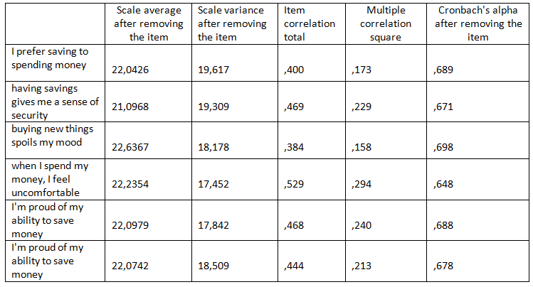
Table 2 shows the statistics for the whole scale when we omit one of the items:
- The first column tells us what the average of the whole scale would be if the statement was removed from the scale. This is calculated by subtracting the average for the item from the average for the whole scale. Of course, one position removed from the scale will always lead to a lower average, even more, the range of possible values will change (a scale consisting of six items can have values from 6 to 36, and a scale consisting of five items - from 5 to 30);
- One item removed from the scale will also reduce variance. The scale variance values after removing each of the items can be found in the second column of the table;
- The third column shows the correlation between the scale item and all the other items taken together. It is calculated as Pearson's R correlation coefficient between the item value and the sum of values of the other items. Generally speaking, when we create a scale, we want the correlation between each element and the whole scale to be high. Otherwise, we may suspect that the item does not measure exactly the same construct as the others and this is a premise for considering the item to be removed from the scale. In our example, the lowest correlation coefficient with the whole scale is for the item buying new things spoils my mood;
- The fourth column shows the multiple correlation square, which you probably know from the R-square regression analysis. For each scale position, a regression model is built in which the item is a dependent variable and all other items assume the role of predictors. The aim is to predict the values for this scale item, based on knowledge of the values of all other items. The higher the R-square, the better;
- The last column of the table contains information about Cronbach's alpha value after deleting the item concerned. As we know from earlier, Cronbach's alpha for the whole scale is 0.71. If it would appear from the table that an item, if removed, would improve (increase) the Cronbach's alpha value, it would be a strong argument for us to reduce our scale down to five items.
- On the basis of previous analyses, we suspected that the statement buying new things spoils my mood may adversely affect the consistency of the scale. Let's see what happens if we remove it. We can read from this table that, after removing this item, Cronbach's alpha value would be reduced, although the decrease would be relatively small. Removing any other position would result in a greater decline. In this case, the final decision is up to the analyst. Perhaps some of you would prefer to leave this variable to maximize Cronbach's alpha. However, if we want our scale not to be too complicated (according to the rule: the simpler, the better), we can decide to remove the item that does not contribute much to our scale.
So let's do the reliability analysis again, but this time with this variable omitted.
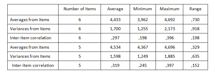
If we look at table 3, we can see that the correlations between the pairs of variables for the 5 items range from 0.245 to 0.397, and the average correlation increased to 0.319. There are also no such large differences between scale items in terms of averages or variances. It seems that it was a good idea to remove the item.

Table 3. Item summary statistics - before and after the removal of the variable “buying new things spoils my mood”
Note, in order to make the scale items similar to each other, we must take care not to exaggerate. Imagine that all scale items are perfectly correlated with each other and have the same averages and variances. In such a situation, the question arises: why construct a scale at all? Instead of analyzing the whole set of variables, it would be enough to choose any one variable from the set. The analysis of this variable would give exactly the same results as the analysis of the whole set. However, in order not to get bogged down in pursuit of excellence, we can use statistical tests available as part of the reliability analysis procedure.
One approach may be to try to match our data to a parallel or closely parallel model. The assumption of the strictly parallel model is that, in the population, all the scale items have the same averages and variances. In the case of the parallel model, the null hypothesis is not so restrictive and only assumes the equality of variance between the scale items. Note that the parallel model is nested in the strictly parallel model: if the assumptions of the parallel model are not met, then it is automatically excluded that the assumptions of the strictly parallel model are met.
Let's try to match the parallel model to our data. Below is a table with the model matching test. This test verifies whether the data allows the adoption of the null hypothesis that there are no differences between the variances of individual scale items.

Tabela 4. Test dla dobroci dopasowania modelu równoległego
A test significance level of less than 0.05 indicates that there are no grounds for adopting the null hypothesis. For us, this means that the variance of at least one item is significantly different from the variance of the other items. If so, it is no longer necessary to perform the matching test for the strictly parallel model.
We already know that the items of our scale do not have equal variance, but what about their averages? In order to check this, we can use tests based on the ANOVA table. These tests allow us to verify the null hypothesis, claiming that the averages of all the items in the population are equal. The selection of the appropriate test depends on the level of measurement of the variables. The F test is used when the variables in the scale are measured on a quantitative level, the Friedman test is used to analyze ordinal variables, and the Cochran test should be selected when the scale is a dichotomy set. Our scale consists of items measured on the ordinal level, so I choose the Friedman test.
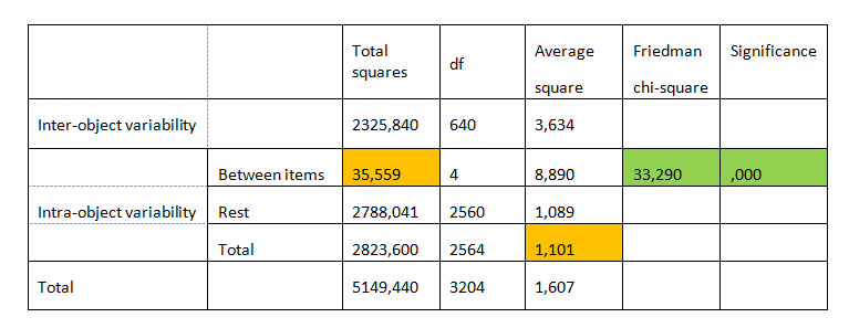
In Table 5 we can read the value of Friedman's chi-square test. This is the ratio of the sum of the squares between the items (35,559) and the average intra-object square (1,101).

Tabela 5. ANOVA with Friedman test
The significance level of the test is smaller than 0,05. Consequently, there is no basis for adopting the null hypothesis. This means that the average of at least one item differs significantly from the other averages.
Statistical tests (both the parallel model matching test and the ANOVA table-based test) have assured us that, although the scale is consistent, we have not exaggerated in our efforts to achieve this consistency. It cannot be said that all scale items carry exactly the same information. Using only one selected variable instead of the whole scale would result in any additional information provided by the other scale items being lost.
In this post, after considering the arguments for and against, we have decided to remove one of the items from our scale. We also performed statistical tests to check the hypotheses about the equality of averages and variance between the items. All this together has allowed us to recognize that our scale will be a good reflection of the bank customers' attitude to saving money.